Controlling the Inverted Pendulum. Example of a Digital Feedback Control System.

CONTROLLING THE INVERTED PENDULUM:
An Example of a Digital Feedback Control System.

A free swinging pendulum is inverted so the hinge is at the bottom. The challenge is to move the bottom of the pendulum back and forth to keep the pendulum from falling over.

The hinge at the bottom of the pendulum is attached to a cart which moves back and forth on a track. The cart is connected to wires which are connected to an electric motor. The voltage applied to the electric motor is controlled by a computer. The observable properties are the current pendulum's angle from vertical and the current cart position.

Below is a diagram of the setup:

This paper derives all the characteristic equations of motion for an inverted pendulum, all the transfer functions, Bode plots, state space representations, and concludes with an example of controlling a real setup.

After mastering this 2-dimensional problem you can expand this to a 3-dimensional problem. If you can master the task of controlling an inverted pendulum free to fall in any direction, then you can launch a rocket into outer space, controlling the thrust angle at the bottom so it doesn't fall over.

EQUATIONS OF MOTION: The Inverted Pendulum
EQUATIONS OF MOTION: The Free Hanging Pendulum
EQUATIONS OF MOTION: The Cart and Motor
CONTINUOUS TIME TRANSFER FUNCTIONS
1. Block Diagram
2. DERIVATION OF STATE SPACE REPRESENTATION
  - State space equations for the cart and inverted pendulum
  - Calculation of Transfer Functions from State Space Equation
DISCRETIZATION OF CONTINUOUS TIME STATE SPACE EQUATIONS
FEEDBACK
CONTROLLING THE PENDULUM: AN EXAMPLE
LINKS FOR FURTHER RESEARCH

THE INVERTED PENDULUM AND CART SYSTEM

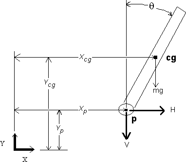
EQUATIONS OF MOTION: The Inverted Pendulum

cg	=	Center of gravity
p	=	Pivot point

	=	X coorordinate of center of gravity

	=	First derivative of

	=	Second derivative of

	=	Y coorordinate of center of gravity

	=	First derivative of

	=	Second derivative of

	=	X coordinate of pivot point.
		Note positive is toward right.

	=	First derivative of

	=	Second derivative of

	=	Y coordinate of pivot point.

	=	First derivative of

	=	Second derivative of
H	=	Force in Horizontal direction.
V	=	Force in Vertical direction.
	=	1/2 length of pendulum
m	=	mass of pendulum
	=	Angle of pendulum measured from vertical.
		Note positive is taken as clockwise.
	=	Viscous damping constant.
I	=	moment of inertia for pendulum ( for uniform rod)

EQUATIONS OF MOTION: The Inverted Pendulum

Coordinates of point cg in terms of point p, angle

, and length

Sum of forces in X direction

Sum of forces in Y direction

Sum of moments about center of gravity

Combine Equations

Assume pendulum is uniform rod with moment of inertia mip

Also assume small angle approximations sin(

) =

, cos(

) = 1

Let

This is our characteristic equation of motion for the inverted pendulum.

TRANSFER FUNCTIONS

In control theory, functions called "transfer functions" are very often used to characterize the input-output relationships of linear time-invariant systems. The concept of transfer functions applies only to linear time-invariant systems, although it can be extended to certain nonlinear control systems.

Transfer Functions. The transfer function of a linear time-invariant system is defined to be the ratio of the Laplace transform of the output (response function) to the Laplace transform of the input (driving function), under the assumption that all initial conditions are zero.

The transfer function is an expression relating the output and input of a linear time-invariant system in terms of the system parameters and is a property of the system itself, independent of the driving function. The transfer function includes the units necessary to relate the input to the output; however, it does not provide any information concerning the physical structure of the system. (The transfer functions of many physically different systems can be identical.)

By using this concept, one can represent the system dynamics by algebraic equations in S.
—Modern Control Engineering by Katsuhiko Ogata, pg. 72. (University of Minnesota.) (©1970)

Derivation of Transfer Function for the Inverted Pendulum

Starting with our characteristic equation from the previous page:

p2_9

we take the Laplace Transform of both sides:

p3_2

and do some rearranging:

p3_3

This is our transfer function for the inverted pendulum.

EQUATIONS OF MOTION: The Free Hanging Pendulum

cg	=	Center of gravity
p	=	Pivot point

	=	X coorordinate of center of gravity

	=	First derivative of

	=	Second derivative of

	=	Y coorordinate of center of gravity

	=	First derivative of

	=	Second derivative of

	=	X coordinate of pivot point.
		Note positive is toward right.

	=	First derivative of

	=	Second derivative of

	=	Y coordinate of pivot point.

	=	First derivative of

	=	Second derivative of

H	=	Force in Horizontal direction.
V	=	Force in Vertical direction.
	=	1/2 length of pendulum
m	=	mass of pendulum
	=	Angle of pendulum measured from vertical.
		Note positive is taken as clockwise.
	=	Viscous damping constant.
I	=	moment of inertia for pendulum ( for uniform rod)

Coordinates of point cg in terms of point p, angle

, and length

Sum of forces in X direction

Sum of forces in Y direction

Sum of moments about center of gravity

Combine Equations

Assume pendulum is uniform rod with moment of inertia

Also assume small angle approximation sin(

) =

Let

This is our characteristic equation of motion for the free hanging pendulum. Compare it with the characteristic equation for the inverted pendulum.

Solution of characteristic equation of motion for the free hanging pendulum

Assume a solution of the form

Let

	=

	=

	=

	=

	=

Here

, and B are constants dependant upon initial conditions. In general the response thetat

will be damped sinusoidal oscillations with a frequency omegd2p

and damping envelope of dampenvl

Determination of Pendulum Parameters

, and

Remove the pendulum assembly from the cart and turn it upside down, allowing the pendulum to hang freely. Start the pendulum swinging and record the position

on a chart recorder. From our previous analysis we expect the response to be something like:

sindamp

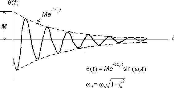
The response will be damped sinusoidal oscillations with a frequency omegd2p

and a damping envelope of dampenvl

From your chart recording estimate the parameters zeta

,and

When I performed this experiment I found the decay appeared to be linear rather than exponential. It appeared the pendulum lost a fixed amount of energy every swing regardless of how wide the swing was.

viscous4

My guess is at the end of each swing when the pendulum momentarily stops the friction changes from kinetic (moving) friction to static (non-moving) friction, and it takes a certain amount of energy to overcome this static friction. zeta

was estimated to be insignificantly small (0.02 as I recall, and I think we set zeta

to zero to simplify the equations later on and ignored the static friction energy loss problem).

EQUATIONS OF MOTION: The Cart and Motor

	=	input voltage. Positive input voltage moves cart toward right.
	=	output voltage
E	=	EMF across motor
	=	Motor armature resistance
	=	Motor armature current
	=	Torque developed by motor
F	=	Force transmitted to wire by motor
	=	Motor shaft angle
r	=	effective radius of motor shaft. ( )
H	=	Force in Horizontal direction.
	=	X coordinate of cart. Note positive is toward right.
	=	Amplifier gain constant
	=	A constant of the motor
M	=	mass of cart
	=	viscous damping of motor
	=	viscous damping of cart
	=	inertia of motor
J	=	combined inertia of motor and cart. ( )
B	=	combined damping of motor and cart. ( )
	=	Viscous damping constant. ( )

THE CART AND MOTOR

Basic Equations of Motor and Amplifier

Combine Equations

Calcuate Torque

Assume m<<M

p10c5

Substitute back in

Observe Following Relations

Substitute in

Let

This is our characteristic equation of motion for the cart and motor system.

Determination of Parameters for the cart and motor

Now take the Laplace Transform of both sides of the characteristic equation on the previous page and rearrange to get the transfer function for the cart and motor.

The transfer function for the cart and motor is:

p11d4

We shall experimentally determine the unknown parameters ksubc

and B. The standard method for doing this is to input sinusoids of various frequencies into the system and make a Bode plot of the resulting output. We expect the Bode plot to have a breakpoint at the frequency corresponding to the unknown parameter B. The equations which predict this response are derived below.

Let p13_2

Here A is the amplitude of the sine wave we are inputting to the system and

is the frequency in radians of the oscillations.

Taking the Laplace transform of both sides gives:

p13_3

Applying this as the input to the transfer function gives:

Expanding by partial fractions:

p13_6

Thus:

Taking the inverse Laplace transform gives:

The last term dies away as times increases, so we are left with a steady state solution of:

p13_13

For those interested: Repeat the above derivation for an input of p13_14

Explain the differences in the results.

The Bode Plot

When we perform the preceding experiment the output we measure is a voltage vsubx (t) which is related to the cart position X(t) by the equation:

Thus our steady state output for an input

acoswt

We now wish to make a Bode plot of the magnitude (in decibels) of the output voltage corresponding to the cart position versus the frequency (in radians) of the input. The magnitude in decibels of vsubx

(t) is

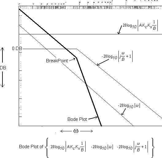
The Bode plot thus consists of three parts. First there is a constant gain term of p15_7a

This is a horizontal line on the Bode plot. Second, there is a pole at the origin with a gain of p15_7b

This is a line with slope of -20 DB/decade with a value of 0 DB at omega

= 1 rad/sec. Third, there is a pole on the real axis at -B given by the term p15_7c

The magnitude of this at low frequencies is:

			()

and at high frequencies the magnitude is:
			()

DETERMINATION OF THE PARAMETERS FOR THE CART AND MOTOR

The first is a horizontal line at 0 DB. The second is a line of slope -20 DB/decade which crosses 0 DB at omega

= B. We thus expect the Bode plot we obtain experimentally to be the sum of the three individual responses. We expect it to look something like the following:

p16_1

DETERMINATION OF PARAMETERS FOR CART AND MOTOR: SQUARE WAVE INPUT

Square Wave Input: For omegaltb

Due to static friction inherant in the cart and motor system it is difficult to obtain an accurate Bode plot when pure sinusoidal inputs are used. When the voltage to the motor is near zero the system tends to stick and not move at all. To overcome this problem we will use a square wave input instead of a sine wave input. We now examine the response we expect to get using a square wave input.
A square wave of frequency

can be expressed as the sum of sine waves as follows:

p17_1

Since our transfer function for the cart and motor is linear, the output due to a square wave is the sum of the outputs due to each of the sinusoudal terms which make up the square wave.

From our earlier analysis we know the magnitude of the output oscillations due to an input of asinwt

is:

For

this becomes

p17_3

For a square wave input expressed as the sum of a series of sinusoidal inputs the magnitude of the output becomes:

		→

		→

			Note: (Proof)

		→

We thus expect the output due to a square wave input to be about 1.233 times the output due to a sine wave input when ( omegaltb

)

Expressed in decibels this becomes:

	DB	=

		=

		=

The output due to a square wave input is about 1.82 DB greater than it would be for a sine wave input when ( omegaltb

)

Solution to series 1 + 1/(3^2) + 1/(5^2) + 1/(7^2) + 1/(9^2) + ...

> solution to this series:
>
> 1 + 1/(3^2) + 1/(5^2) + 1/(7^2) + 1/(9^2) + ...

See: http://www.efunda.com/math/seriesofconst/IntRecipSeries.cfm

Or:
Let A = 1 + 1/(3^2) + 1/(5^2) + 1/(7^2) + 1/(9^2) + ...

Using the Riemann's Zeta Function and its 'alternating' form
 Zt(s) = Sum_{n=1}^\infty [ 1/n^s ]
 Za(s) = Sum_{n=1}^\infty [ (-1)^{n-1} / n^s ]
       = [ 1 - 2^{1-s} ] Zt(s)

It is easy to verify that
 A = [ Zt(2) + Za(2) ] / 2
   = (1/8)pi^2

There are around half-dozen proofs that Zeta(2) = pi^2/6.

========================

Or:
Here is a proof using Fourier series:

Take the function fx(x)	= -x	when -π < x < 0
	= 0	when 0 < x < π

Notice f(x) is piecewise continuous with period 2π so this means we can find its corresponding Fourier series.

Solve for the coefficients of the Fourier series, and write out the Fourier series for f(x)

f(x) = π/4 - (2/π)*[cos(x) + (1/9)cos(3x) + (1/25)cos(5x) ...] - [sin(x) - (1/2)sin(2x) + (1/3)sin(3x) ...]

Now just evaluate at x=0

You get

0 = π/4 - 2/π * (1 + 1/9 + 1/25 +...)

so π²/8 = (1 + 1/9 + 1/25 + ...)

Square Wave Input: For omegagtb

We now examine what happens when omegagtb

For

our output due to a sine wave input becomes:

p18_10

For a square wave input expressed as the sum of a series of sinusoidal inputs the output becomes:

			→

			→

			→

We thus expect the output due to a square wave input to be about 1.052 times the output due to a sine wave input. Expressed in decibels this becomes:

	DB	=

		=

		=

The output due to a square wave input is about 0.44 DB greater than it would be for a sine wave input when omegagtb

We may conclude that the difference in response between a sine wave input and a square wave input is small. Thus, to experimentally determine the unknown parameter B we may use square waves of various frequencies and analyze the results the same as we would for a sine wave input.

BLOCK DIAGRAM

TRANSFER FUNCTIONS

			(The Inverted Pendulum)

			(The Cart and Motor System)

We will later use the variables xsubp

(t),

(t),

(t) as the state space variables for our state space representation of the system. We can show the Laplace transform of these variables on the block diagram as follows:

p19_2

Derivation of State Space Representation

Equation of motion for the cart

(Our characteristic equation of motion for the cart and motor system derived earlier.)

(Solve for xdot2p

)

Equation of motion for the Inverted Pendulum

(Our characteristic equation of motion for the inverted pendulum derived earlier. Now solve for

)

State Space Representations


			(Equation of motion for the cart derived above)

			(Equation of motion for the inverted pendulum derived above)

This can be represented in matrix form as:

p20c5

This has the general form of:

p20d1

Calculation of Transfer Functions from State Space Equation

For the moment we assume all four of the state space variables are individually observable. Thus:

p21a1

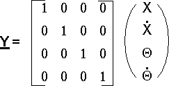
This has the form p21a2

where C = I, the identity matrix

The transfer function matrix is given by:

F(s) = C p21sia

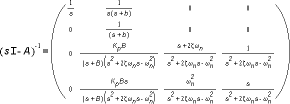
Calculate where I is the identity matrix, and A was the 4x4 matrix derived two pages ago under Derivation of State Space Representation.

Calculate F(s) = CB where C = I, the identity matrix, and B is the vector derived three pages ago at the bottom under Derivation of State Space Representation.

F(s) = CB

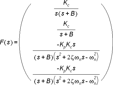
Recall from earlier the transfer function equations:

		Transfer function for the cart and motor system.

		Transfer function for the inverted pendulum.

And recall from the Laplace transform that p22_7

= s

[f(t)]

Thus p22_4

and

Our equation F(s) is now:

p22_6

Discretization Of Continuous Time State Space Equations

where

Calculation of G

Calculation of inverse Laplace Transforms

We now have the arduous task of calculating the inverse Laplace transform for the terms in the 4x4 matrix on the previous page.

Going down the rows we have

Row 1, Column 1

pm11_1

Row 1, Column 2

Row 2, Column 2

Calculation of inverse Laplace Transform for row 3 column 2.

when

= 0 and

Substituting these values of asub1

and

into equations N1, N2, N3 on the previous page gives

pm32_2a

Substituting these values of nsub1

, and

into equation L4 on the previous page gives the Laplace transform of row 3 column 2 as

pm32

which reduces to

pm32r

Calculation of inverse Laplace Transform for row 4 column 2.

when

= 0 and

Substituting these values of asub1

and

into equations N1, N2, N3 derived two pages ago gives

pm42_2a

Substituting these values of nsub1

, and

into equation L4 derived two pages ago gives the Laplace transform of row 4 column 2 as

pm42

which reduces to

pm42r

Calculation of inverse Laplace Transform for (row,column) (3,3) (3,4)(4,3) (4,4)

A general form of these equations is

pm33g_4

(We will save nsub1

for later use.)

Extract nsub2

from top and factor the bottom

pm33g_5

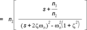
Add

to top

Split top

Multiply second term by pm33g_8j

Taking the inverse Laplace transform of the above equation gives

pm33g_9

EQUATION L5

pm33g_10

Calculation of inverse Laplace Transform for row 3 column 3.

when

= 1 and

Substituting these values of nsub2

and

into equation L5 derived on the previous page gives the Laplace transform of row 3 column 3 as

pm33

which slightly reduces to

pm33s

Calculation of inverse Laplace Transform for row 3 column 4.

when

= 0 and

= 1

Substituting these values of nsub2

and

into equation L5 gives the Laplace transform of row 3 column 4 as

pm34

Calculation of inverse Laplace Transform for row 4 column 3.

when

= 0 and

Substituting these values of nsub2

and

into equation L5 gives the Laplace transform of row 4 column 3 as

pm43

Calculation of inverse Laplace Transform for row 4 column 4.

when

= 1 and

= 0

Substituting these values of nsub2

and

into equation L5 gives the Laplace transform of row 4 column 4 as

pm44

Calculation of G

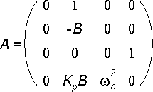
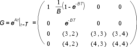
where
(3,2) = pm32r

(4,2) =

(3,3) =

(3,4) =

(4,3) =

(4,4) =

Calculation of G assuming zeta

= 0

If our damping factor for the pendulum zeta

is estimated to be small enough that we can set it to zero then our equations simplify to

draft23

where
(3,2) = pmz32

(4,2) =

Calculation of H when zeta

, = 0

rearanging gives

p30_3

Discussion of Observable Properties

The two state veriables X and

are directly observable by measuring the voltage from the corresponding potentiometers and multiplying by appropriate scaling constants. Thus:

p32a_1a

;

= Voltage corresponding to X position p32a_1c

;

= Voltage corresponding to X position p32a_2c

For the moment we will assume the other variables xdot

and

are also directly observable. Thus our output vector Y consisting of observable states of the system becomes:

p32a_3

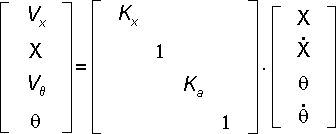
which has the form

p32a_4

Discussion of Feedback

We now decide to use a linear combination of the observable states contained in vector y to determine the input controlling voltage.

p32b_1

= KY

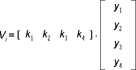
Our original state space equation was

x(k+1) = Gx(k) + Hv(k)

y = Cx(k)

Now observe that our input v(k) is actually vsubi

, the input controlling voltage to the servo motor. We also have decided to set vsubi

= KY, and we know y = Cx(k) Thus we now have:

x(k+1) = Gx(k) + HkCx(k)

x(k+1) = (G + HkC)x(k)

p33_5

Note that in this case HK is the outer product of two vectors producing a square matrix.

If we assume an initial x vector x(0), we then have

p33_6

As k increases, the components of vector x(k) will tend toward zero only if the eigenvalues of the matrix (G + HKC) all have magnitude less than one. It is now our job to chose the four values, p33_7

such that the matrix (G + HKC) is stable.

Procedure to obtain ksubx

Measure voltage vsubl

from position potentiometer. Move cart one meter to right and measure voltage vsubr

from position potentiometer.

p34a_1

Procedure to obtain ktheta

Lay pendulum at -90 degrees horizontal with table, pendulum pointing left. Measure vsubl

from pendulum angle potentiometer. Turn pendulum 180 degrees (

radians) clockwise (positive sense) so pendulum is horizontal with table, pointing right. Measure vsubr

from pendulum angle potentiometer.

p34b_1

BLOCK DIAGRAM OF SYSTEM WITH DISCRETE-TIME FEEDBACK

Motor Dead Range

Due to static friction the servo motor has an input voltage threshold below which the motor will not move. The friction is primarily due to the brushes within the servo motor. A graph of the input voltage versus cart velocity might look something like the following:

To compensate for this non-linearity we can add to our calculated control voltage the corresponding threshold voltage. If the calculated control voltage is positive we add the threshold voltage to the control voltage to compensate for the deadrange, and if the calculated voltage is negative we add a negative threshold voltage to the control voltage to compensate for the deadrange. A graph of the transfer function would look something like:

Note that this function is the inverse of the previous function. It thus cancels out the non-linearity of the motor-cart system due to static friction making the system appear more linear.

BLOCK DIAGRAM OF SYSTEM WITH DISCRETE-TIME FEEDBACK AND MOTOR DEADSPACE CANCELATION

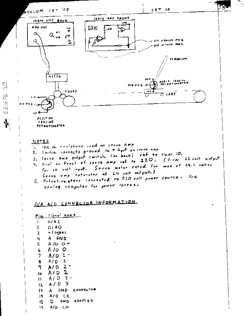
PENDULUM SETUP

Parameters for the Cart and Motor

The response of the cart and motor system to square wave inputs of frequencies 0.1 Hz to 15 Hz was recorded on the chart recorder and plotted on a Bode plot. The primary breakpoint between the line of slope -20 Db/decade and the line of -40 Db/decade occurred at 1 Hz (or omega = 6.28 rad.) A secondary breakpoint of unknown origin occurred at 7 Hz.

The cart gain constant ksubp was obtained by analyzing the magnitude of the cart oscillations for low frequencies. Using the equation

the value of ksubc

was determined by assuming the cart acceleration xdot2p

was zero for low frequencies and then calculating the average velocity xdot1p

from the chart recorder.

COMPLETE LIST OF PARAMETERS

The following parameters were determined by experiment:

omegad

= 5.41 rad/sec
zeta

= 0

= 5.41 rad/sec
ksubp

= 3 1/meter
beta

= 6.28 rad/sec
ksubc

= 1.5

= 6.75 volts/meter
ktheta

= 3.34 volts/meter
T = 0.06 1/sec

CONTROL OF THE PENDULUM

Determination of Feedback Control Parameters

Two computer programs were written to aid in the selection of feedback control values. The first program, ACKERMAN, calculates the control vector K given the desired pole positions using Ackerman's formula. The second program, PENDULUM, does the reverse; it calculates the pole positions given a control vector K.

Control of the Pendulum

Various values of the control vector K were obtained using program ACKERMAN. The final control vector used was X = 3.5, xdot

= 7.0,

= 25.0,

= 3.0 Using these values the poles were calculated to be at 0.752 plusormi

0.382j, 0.929, 0.982

Using these values the pendulum remained upright with the cart slowly oscillating back and forth covering a distance of about 25 cm. The cart was run for a period of 2 minutes and showed no signs of instability.

Analysis of the Results

In a final effort to justify the endless hours spent in deriving a theoretical analysis of the pendulum system, it is gratifying to be able to sit back and say IT WORKS!

(If you've been paying attention you may have noticed that two of the poles were at 0.929 and 0.982, which is pretty close to being unstable. The reason is I initially made a mistake calculating the control values because I used the full length of the rod for

when

was originally defined as 1/2 the length of the rod. Recalculating using the correct value for

gave the true poles.)

Links For Further Research

There's been further research since this paper was originally written in 1987. My thanks to Reid Sweatman for providing the following comments and links:

Curious side note: this problem is susceptible to fairly easy solution by neural net, and as such, is an example problem in several texts, sometimes slightly modified to balance the stick upright, rather than oscillate it. Of course, this removes a number of exponential terms from the differential solution, but, strangely enough, that doesn't make much difference to the neural net solution, beyond requiring extra feed-forward layers.

I believe a genetic algorithm might also be capable of handling the problem, so long as it was updated often enough to keep the stick reasonably within the solution space. However, I've never seen that done, or tried it myself. I do neural nets more frequently than genetic algorithms, but have a friend who has done several exceedingly complex game AIs (essentially very complex routing schedulers) who maintains it's possible. I suppose of equal interest is the frequency with which AIs are simulated by physical systems, like constrained springs.

I've got two favorite books on neural nets:

Neural Networks: A Comprehensive Foundation, by Simon Haykin, and
Neural Smithing: Supervised Learning in Feedforward Artificial Neural Networks, By Russell D. Reed and Robert J. Marks II

For a web site, you can't do much better for a launch point than Steve Woodcock’s site,. Lots of good stuff there. Lots of really funny things (check the "You know your game is in trouble when..." page), and links to just about everything in AI. Although the site is dedicated to AI in computer games, Steve works for Raytheon doing, last I talked to him, missle guidance systems. Before his brief sojourn into gaming, he wrote AI code for Star Wars (not the movie one). I think he still co-chairs the AI roundtable discussions at the annual Computer Game Developers' conference in San Jose, as well as a more academic one just up the road about two weeks later. Those roundtables are the thing I always like best about the GDC, although I haven't been since 2000. Hey, where else can you get a few hours of what's essentially free consulting with guys like Steve and Neil Kirby from Lucent on your game AI? Hashed out a messy flocking/steering infantry AI with Steve, then the same for training a neural net flight simulation pilot later that night with Neil. Keeps the old brain cells in motion.